Code & Implementation

Canadian National Broadcast Company showing their sources of funding in two financial years.

Redesign 1

library(tidyverse)
library(plotly)
library(lattice)

Sources_of_Funding <- c('Government_Funding', 'Revenue', 'Financing_and_Other_Income',
       'Subscriber_Fees', 'Advertising', 'Digital', 'Television')

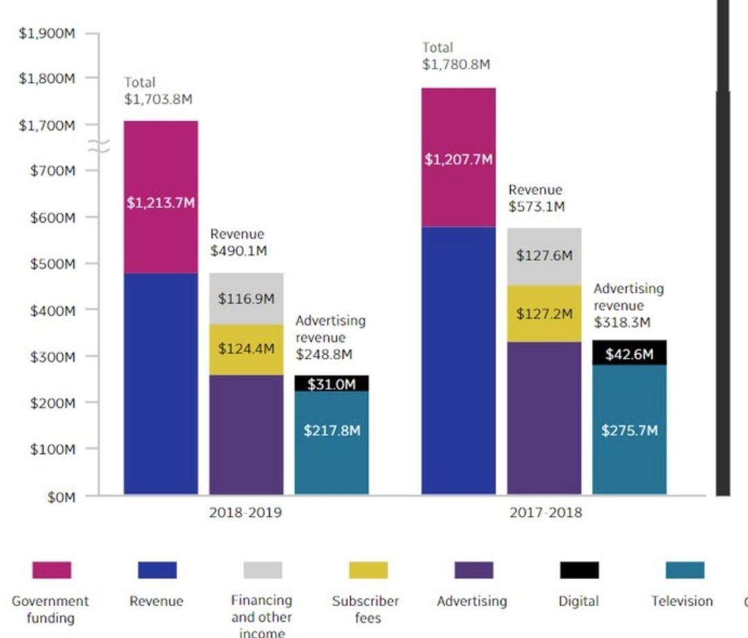
Year1_Funding <- c(1207.7,573.1,126.6,127.2,318.3,42.6,275.7)
Year2_Funding <- c(1213.7,490.1,116.9,124.4,248.8,31.0,217.8)

m <- list(
  l = 50,
  r = 50,
  b = 50,
  t = 70
)

Funding <- data.frame(Sources_of_Funding, Year1_Funding, Year2_Funding)
Funding

          Sources_of_Funding Year1_Funding Year2_Funding
1         Government_Funding        1207.7        1213.7
2                    Revenue         573.1         490.1
3 Financing_and_Other_Income         126.6         116.9
4            Subscriber_Fees         127.2         124.4
5                Advertising         318.3         248.8
6                    Digital          42.6          31.0
7                 Television         275.7         217.8

Plot1 = plot_ly(Funding, y = ~Sources_of_Funding, x = ~Year1_Funding, type = 'bar', name = '2017-2018',marker=list(color = 'red')) %>% 
    add_trace(x = ~Year2_Funding, name = '2018-2019', 
              marker = list(color = 'blue')) %>%
    layout(title= list(text="<b> Canadian National Broadcast Company showing\ntheir sources of funding in two financial years. </b>",x=0.5,y=0.9,xanchor='center',yanchor='top'),font=list(size=10))  %>%
    layout(legend= list(title=list(text='<i><b>Year</b></i>'),x=100,y=0.5),
           xaxis = list(title = "<b>Funds in Millions<b>",
                   tick0=0, dtick=250,font=list(size=8.5)),
           yaxis = list(title = "<b>Source of Funding</b>",font=list(size=8.5)),
           margin = m,
           barmode='group')

Plot1

Redesign 2

Year                       <- c("2017-2018", "2018-2019")
Government_Funding         <- c(1207.7, 1213.7)
Revenue                    <- c(573.1, 490.1)
Financing_and_Other_Income <- c(126.6, 116.9)
Subscriber_Fees            <- c(127.2, 124.4)
Advertising                <- c(318.3, 248.8)
Digital                    <- c(42.6, 31.0)
Television                 <- c(275.7, 217.8)

mat <- data.frame(Year, Government_Funding,Revenue,Financing_and_Other_Income,Subscriber_Fees,Advertising,Digital,Television)
mat 

       Year Government_Funding Revenue Financing_and_Other_Income
1 2017-2018             1207.7   573.1                      126.6
2 2018-2019             1213.7   490.1                      116.9
  Subscriber_Fees Advertising Digital Television
1           127.2       318.3    42.6      275.7
2           124.4       248.8    31.0      217.8

Funds = gather(mat,key = Source_of_Funding,value = Funding,Government_Funding:Television,factor_key = T)
Funds

        Year          Source_of_Funding Funding
1  2017-2018         Government_Funding  1207.7
2  2018-2019         Government_Funding  1213.7
3  2017-2018                    Revenue   573.1
4  2018-2019                    Revenue   490.1
5  2017-2018 Financing_and_Other_Income   126.6
6  2018-2019 Financing_and_Other_Income   116.9
7  2017-2018            Subscriber_Fees   127.2
8  2018-2019            Subscriber_Fees   124.4
9  2017-2018                Advertising   318.3
10 2018-2019                Advertising   248.8
11 2017-2018                    Digital    42.6
12 2018-2019                    Digital    31.0
13 2017-2018                 Television   275.7
14 2018-2019                 Television   217.8

Plot2 = ggplot(Funds, aes(x= Funding,y=Year,fill=Source_of_Funding,group = Source_of_Funding)) +
  geom_point(shape = 21, size = 1.5) + 
  geom_line(aes(color = Source_of_Funding)) +
  labs(title="Canadian National Broadcast Company showing their sources of\nfunding in two financial years.",fill="Source of Funding",x="Funds in Millions",y="Year")+
  scale_x_continuous(breaks=seq(0,1250,by=150)) + 
  theme(legend.position ="none",
        plot.margin = margin(t = 25,  
                             r = 5,  
                             b = 5,  
                             l = 6),
        plot.title=element_text(size=10,face="bold",hjust=0.5),
        axis.text=element_text(size=6),
        axis.title=element_text(size=8.5,face="bold"))+
  facet_wrap(~Source_of_Funding)

Plot2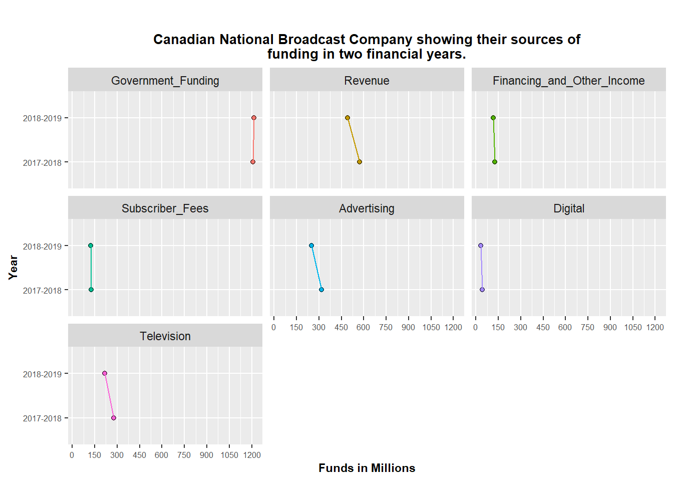

Using ggplotly to make the above graph interactive.

ggplotly(Plot2)