Codes

Research 1:

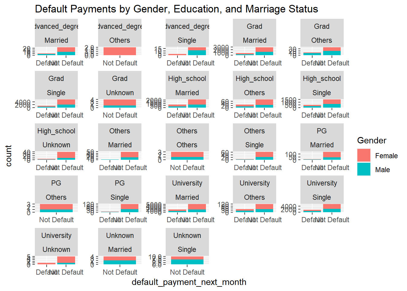
Certain demographic groups have a higher or lower likelihood of defaulting on credit card payments

Code:

# Load necessary libraries
library(readr)  # For data reading
library(dplyr)  # For data manipulation

Attaching package: 'dplyr'

The following objects are masked from 'package:stats':

    filter, lag

The following objects are masked from 'package:base':

    intersect, setdiff, setequal, union

library(ggplot2)  # For data visualization
library(caret)  # For machine learning models

Loading required package: lattice

# Read the dataset
credit_data <- read.csv("C:\\Users\\nmadh\\OneDrive\\Desktop\\Final Project\\Final_output.csv")

# 1. Preprocess the data
# Convert categorical variables to factors
credit_data$Gender <- as.factor(credit_data$Gender)
credit_data$Education <- as.factor(credit_data$Education)
credit_data$Marriage <- as.factor(credit_data$Marriage)
credit_data$default_payment_next_month <- as.factor(credit_data$default_payment_next_month)

# Check for missing values
sum(is.na(credit_data))

[1] 0

# 2. Explore the data
# Visualize default payments across different demographic groups
plot1 = ggplot(credit_data, aes(x = default_payment_next_month, fill = Gender)) +
  geom_bar() +
  facet_wrap(~ Education + Marriage, scales = "free") +
  labs(title = "Default Payments by Gender, Education, and Marriage Status")
plot1

# 3. Train regression models
# Split the data into training and testing sets
set.seed(123)  # For reproducibility
train_index <- createDataPartition(credit_data$default_payment_next_month, p = 0.7, list = FALSE)
train_data <- credit_data[train_index, ]
test_data <- credit_data[-train_index, ]

# Train logistic regression model
logit_model <- glm(default_payment_next_month ~ ., data = train_data, family = binomial)

# 4. Evaluate model performance
# Make predictions on the test set
predictions <- predict(logit_model, newdata = test_data, type = "response")
predicted_classes <- ifelse(predictions > 0.5, "Default", "Not Default")

# Confusion matrix
confusionMatrix(table(predicted_classes, test_data$default_payment_next_month))

Confusion Matrix and Statistics

                 
predicted_classes Default Not Default
      Default        1508        6795
      Not Default     482         214
                                          
               Accuracy : 0.1914          
                 95% CI : (0.1833, 0.1996)
    No Information Rate : 0.7789          
    P-Value [Acc > NIR] : 1               
                                          
                  Kappa : -0.0991         
                                          
 Mcnemar's Test P-Value : <2e-16          
                                          
            Sensitivity : 0.75779         
            Specificity : 0.03053         
         Pos Pred Value : 0.18162         
         Neg Pred Value : 0.30747         
             Prevalence : 0.22114         
         Detection Rate : 0.16757         
   Detection Prevalence : 0.92266         
      Balanced Accuracy : 0.39416         
                                          
       'Positive' Class : Default         
                                          

Research 2:

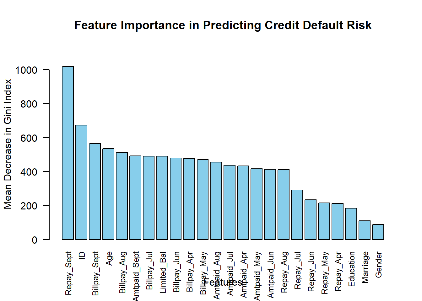
Features that are deemed most important in predicting credit default risk

Code:

data <- read.csv("C:\\Users\\nmadh\\OneDrive\\Desktop\\Final Project\\Final_output.csv")

data$Gender<- factor(data$Gender)
data$Education <- factor(data$Education)
data$Marriage <- factor(data$Marriage)
data$Repay_Sept <- factor(data$Repay_Sept)
data$Repay_Aug <- factor(data$Repay_Aug)
data$Repay_Jul <- factor(data$Repay_Jul)
data$Repay_Jun <- factor(data$Repay_Jun)
data$Repay_May <- factor(data$Repay_May)
data$Repay_Apr <- factor(data$Repay_Apr)
data$default_payment_next_month <- factor(data$default_payment_next_month)

# Load required libraries
library(randomForest)

Warning: package 'randomForest' was built under R version 4.3.3

randomForest 4.7-1.1

Type rfNews() to see new features/changes/bug fixes.

Attaching package: 'randomForest'

The following object is masked from 'package:ggplot2':

    margin

The following object is masked from 'package:dplyr':

    combine

# Set seed for reproducibility
set.seed(1234)

# Train the Random Forest model
rf_model <- randomForest(default_payment_next_month ~ ., data = data)

# Get variable importance measures
importance <- importance(rf_model)

# Sort variable importance measures by importance
var_importance <- importance[order(-importance[, 1]), ]

# Display variable importance measures
print(var_importance)

  Repay_Sept           ID Billpay_Sept          Age  Billpay_Aug Amtpaid_Sept 
  1018.32726    672.52568    563.75433    534.11658    512.46432    493.17382 
 Billpay_Jul  Limited_Bal  Billpay_Jun  Billpay_Apr  Billpay_May  Amtpaid_Aug 
   491.20440    490.99607    478.71140    476.84633    469.35011    455.75366 
 Amtpaid_Jul  Amtpaid_Apr  Amtpaid_May  Amtpaid_Jun    Repay_Aug    Repay_Jul 
   436.19727    433.73568    417.53178    413.28457    410.82039    291.82828 
   Repay_Jun    Repay_May    Repay_Apr    Education     Marriage       Gender 
   234.61829    214.68302    210.96277    184.38949    109.52670     88.19018 

The output shows the importance of different variables in predicting credit default risk. Repayment behavior in previous months, represented by variables like Repay_Sept, has the highest importance, indicating its strong influence on predicting default. Billing and payment amounts also contribute to prediction but to a lesser extent. Demographic variables like Age have some importance, while Customer ID has limited predictive power. Overall, understanding these factors helps in assessing credit risk and making informed decisions.

str(importance)

 num [1:24, 1] 672.5 491 88.2 184.4 109.5 ...
 - attr(*, "dimnames")=List of 2
  ..$ : chr [1:24] "ID" "Limited_Bal" "Gender" "Education" ...
  ..$ : chr "MeanDecreaseGini"

# Extract the values of MeanDecreaseGini
importance_values <- as.numeric(importance[, 1])

# Sort feature importance values in descending order
importance_values_sorted <- sort(importance_values, decreasing = TRUE)

# Get corresponding feature names
feature_names <- rownames(importance)[order(importance_values, decreasing = TRUE)]

# Plot feature importance
barplot(importance_values_sorted, 
        main = "Feature Importance in Predicting Credit Default Risk",
        xlab = "Features",
        ylab = "Mean Decrease in Gini Index",
        cex.names = 0.8,
        las = 2,  # Rotate labels vertically
        col = "skyblue",
        ylim = c(0, max(importance_values_sorted) * 1.1),
        names.arg = feature_names,
        args.legend = list(x = "topright"),  # Adjust x-axis label position
        mar = c(10, 10, 14, 12))  # Adjust margin (bottom margin increased)

Research 3:

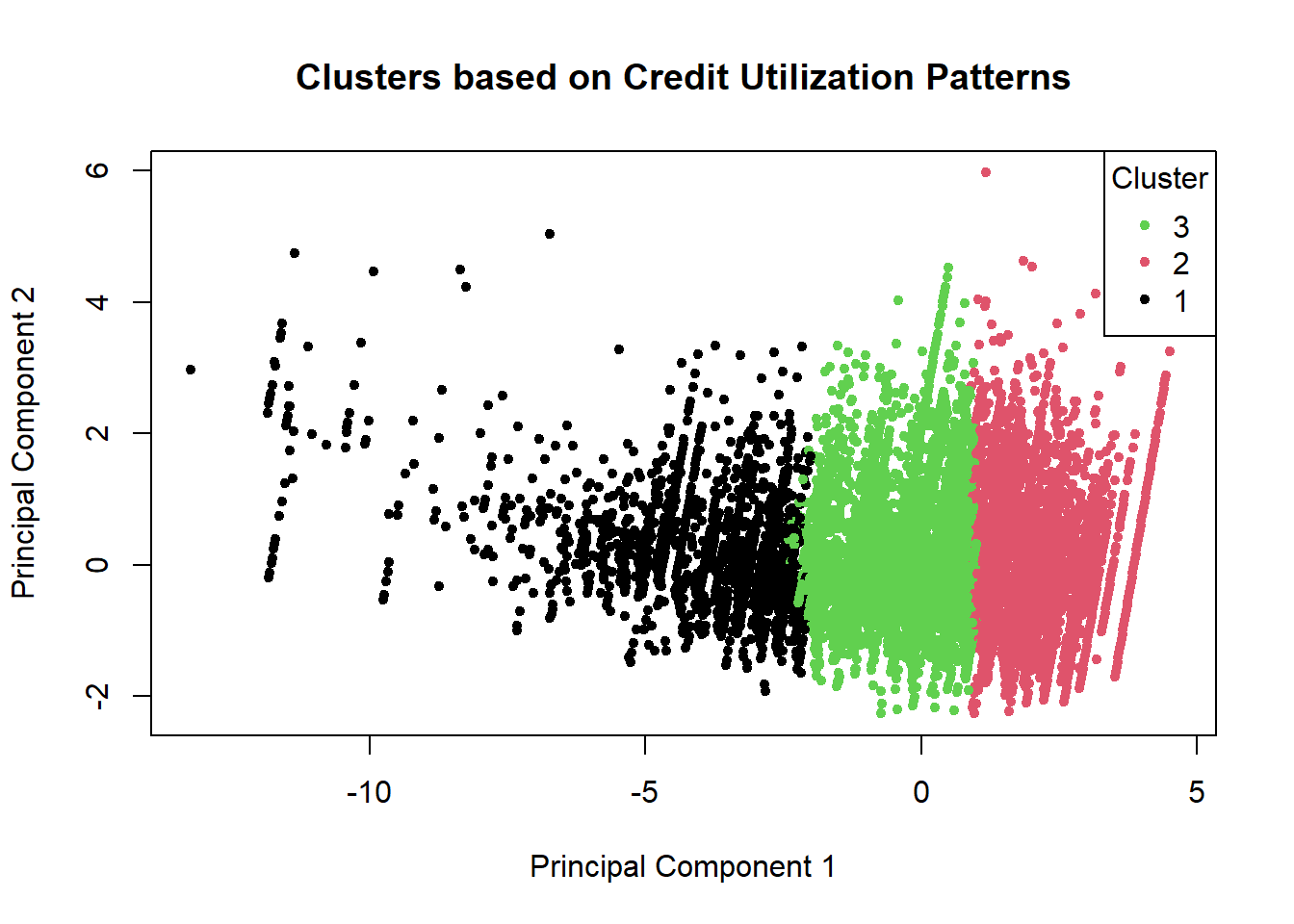
Distinct patterns of credit limit utilization among users.

Code:

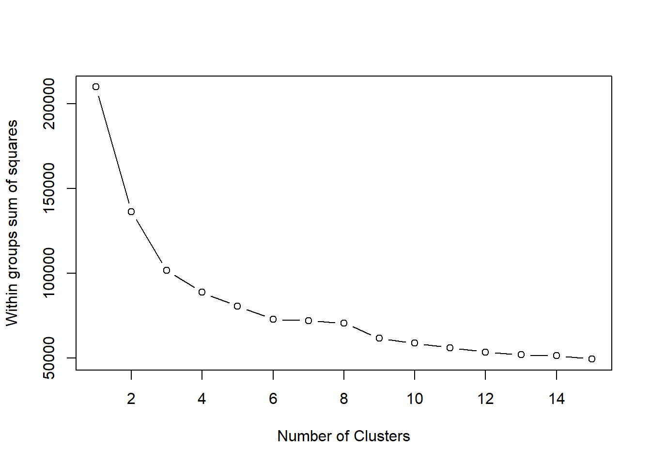
# Load necessary libraries
library(cluster)

# Load the dataset
credit_data <- read.csv("C:\\Users\\nmadh\\OneDrive\\Desktop\\Final Project\\Final_output.csv")

# Step 2: Select relevant columns for clustering
data_for_clustering <- credit_data[, c("Limited_Bal", "Repay_Apr", "Repay_May", "Repay_Jun", "Repay_Jul", "Repay_Aug", "Repay_Sept")]

# Step 3: Standardize the data
scaled_data <- scale(data_for_clustering)

# Step 4: Determine optimal number of clusters using elbow method
wss <- (nrow(scaled_data)-1) * sum(apply(scaled_data, 2, var))
for (i in 2:15) wss[i] <- sum(kmeans(scaled_data, centers=i)$withinss)
plot(1:15, wss, type="b", xlab="Number of Clusters", ylab="Within groups sum of squares")

# Step 5: Based on the elbow plot, select the number of clusters (e.g., 3)
num_clusters <- 3

# Step 6: Perform K-means clustering
kmeans_result <- kmeans(scaled_data, centers=num_clusters)

# Step 7: Assign cluster labels to each user
cluster_labels <- kmeans_result$cluster

# Step 8: Add cluster labels to the original dataset
credit_data_with_clusters <- cbind(credit_data, cluster = cluster_labels)

# Step 9: Get the cluster centers
cluster_centers <- kmeans_result$centers

# Step 10: Calculate standard deviations across columns
col_std_dev <- apply(data_for_clustering, 2, sd)

# Step 11: Scale the cluster centers by dividing by standard deviations
cluster_centers <- scale(cluster_centers, center = FALSE, scale = col_std_dev)

# Step 12: Assign column names to cluster_centers
colnames(cluster_centers) <- colnames(data_for_clustering)

# Step 13: View cluster centers
print(cluster_centers)

    Limited_Bal  Repay_Apr  Repay_May  Repay_Jun  Repay_Jul  Repay_Aug
1 -4.699941e-06  1.2499464  1.4093804  1.4227930  1.4360907  1.4124949
2  3.644460e-06 -0.8264215 -0.8801255 -0.8758454 -0.8553181 -0.8132726
3 -9.206548e-07  0.1728956  0.1688987  0.1641300  0.1511985  0.1346120
   Repay_Sept
1  1.28978602
2 -0.66272483
3  0.08266683
attr(,"scaled:scale")
 Limited_Bal    Repay_Apr    Repay_May    Repay_Jun    Repay_Jul    Repay_Aug 
1.297477e+05 1.149988e+00 1.133187e+00 1.169139e+00 1.196868e+00 1.197186e+00 
  Repay_Sept 
1.123802e+00 

# Visualization (Optional):
# Plot clusters based on the first two principal components
pca_data <- prcomp(scaled_data, center = TRUE, scale. = TRUE)
plot(pca_data$x[, 1], pca_data$x[, 2], col = cluster_labels, pch = 20, main = "Clusters based on Credit Utilization Patterns", xlab = "Principal Component 1", ylab = "Principal Component 2")
legend("topright", legend = unique(cluster_labels), col = unique(cluster_labels), pch = 20, title = "Cluster")